Usage Information
The Smart Geiger-Müller Sensor consists of the GM tube, and a steel rod for clamping it to suitable mounting for ease of use. This device allows the quantification of ionising events generated by a radioactive source. Connecting the sensor to the EasySense app allows data collection.
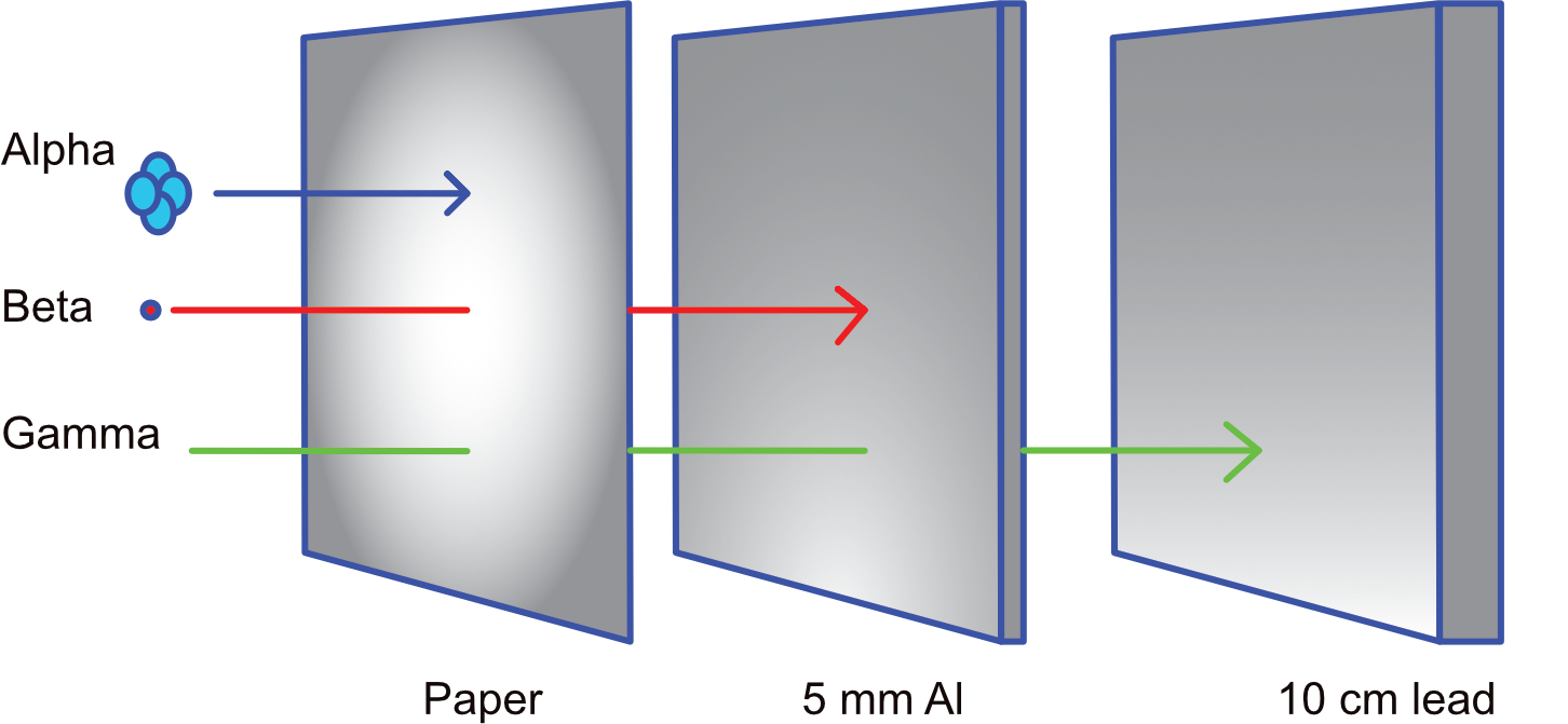
A Geiger-Müller (GM) tube monitors alpha, beta, and gamma radiation. The penetration properties of alpha, beta and gamma are quite different. The GM tube can record single instances of these. The GM tube will register and count events from sources that give rise to ionisation within the GM tube.
It is possible to use the GM tube to count events that emanate from a radioactive source of interest. Additionally, the generalised properties of radiation and their relative contributions may be recorded. A GM tube can also be used to look at the changes, in time, from a radioactive source and the general rules that define radioactive source behaviour.
GM Tube Sensitivity Overview
Sensitivity depends on:
Type of GM tube
Tube voltage (typically recommended: 500V)
Energy of the radiation source
Gamma radiation often results in lower sensitivity.
Handling Low Sensitivity
There are two recommended approaches:
Option 1: Experimental Adjustment
Increase the count interval (measurement time). This improves statistical reliability and works well for inverse square law experiments.
Decrease distance to the source. Be cautious: At very short distances, the finite window size of the tube affects accuracy (the emission becomes non-uniform across the sensor window).
Note for decay rate experiments: Using longer intervals may distort the calculated decay constant due to averaging over decaying activity.
Option 2: Apply a Conversion Factor
Use a scaling correction to adjust the measured count rate to match expected values. In EasySense2, use the "ax" function, "a" = correction factor.
E.g., if the GM tube only detects 10%, use a = 10
If the original counts are statistically weak, scaling won't improve statistical quality, it just amplifies noise!
Additional Considerations
When adjusting distance or interval, ensure that radiation dose remains within safe and recommended limits. Always document adjustments and corrections for transparency and reproducibility.
Theory
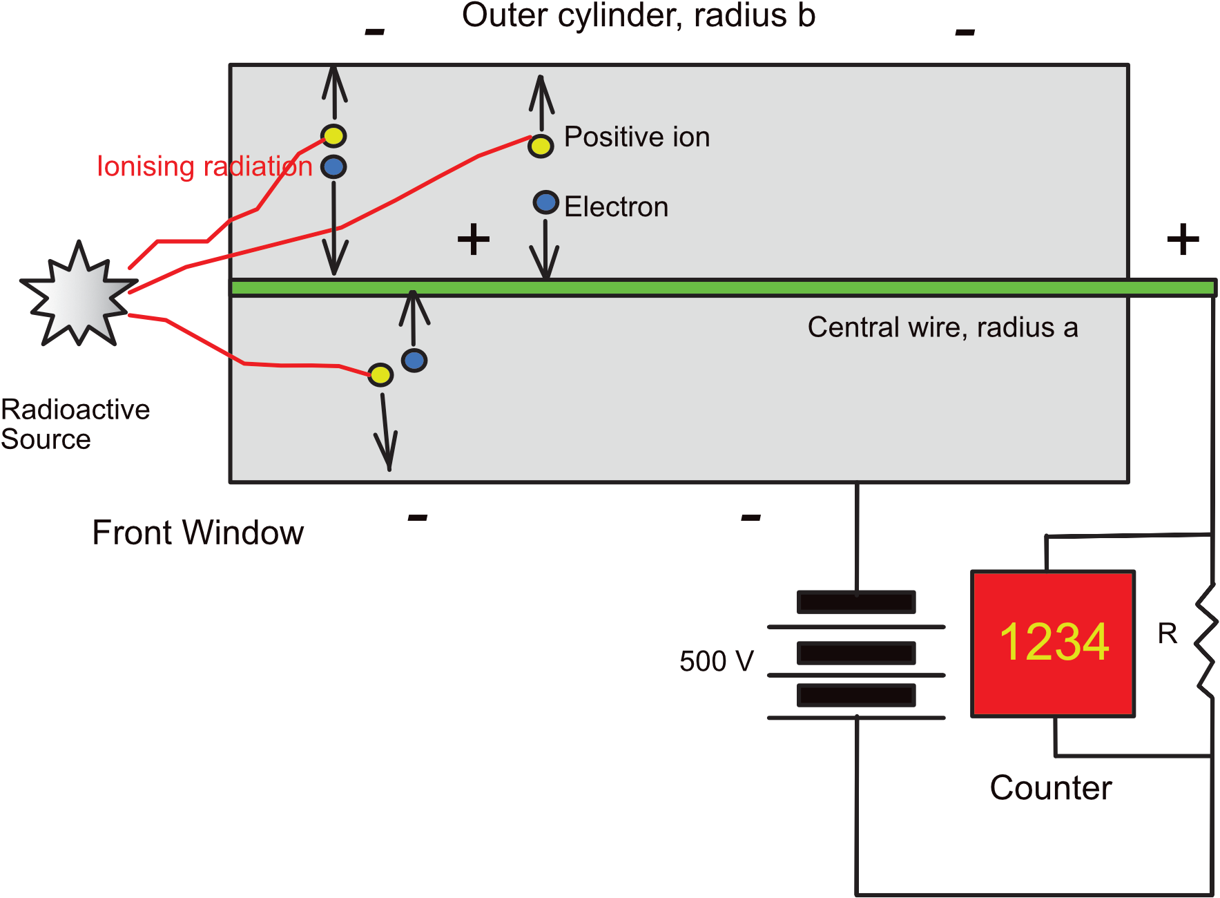
The Smart Geiger Müller Sensor is a GM tube with built-in power supply and associated electronics. It is a gas-filled tube (0.1 atmosphere) that uses a voltage of around 500 V, applied to its positively charged inner wire. It has associated electronics to count “bursts of electrons” that result from ionisation from a radioactive source.
When ionising radiation enters the GM tube window, it displaces electrons from the gas (ionises), which in turn accelerate to toward the inner wire. These displace more electrons on their journey. What results is an “avalanche of electrons.” The electrons flow to the positive voltage and are counted as electron bursts. Each burst represents a single event. The positively charged gas atoms, flow to the outer cylinder wall, and recombine with electrons to replenish the noble gas supply.
The GM sensor is an especially useful device and can help demonstrate interesting and important principles in radiation science.
The GM tube will output a pulse. This output does not depend upon the energy of the radiation that enters the tube. All that is needed is for excitation to be great enough to be able to reach the detection region and to produce subsequent ionisation.
Each GM tube must be set to the correct voltage (circa 500 V) so that an event is detectable. If the voltage is too little, the avalanche will not result. If the voltage is too much, then gas breakdown will occur and hide the event. The Smart Geiger-Müller Sensor is a GM tube is controllable to facilitate the optimal performance for radioactive source studies.
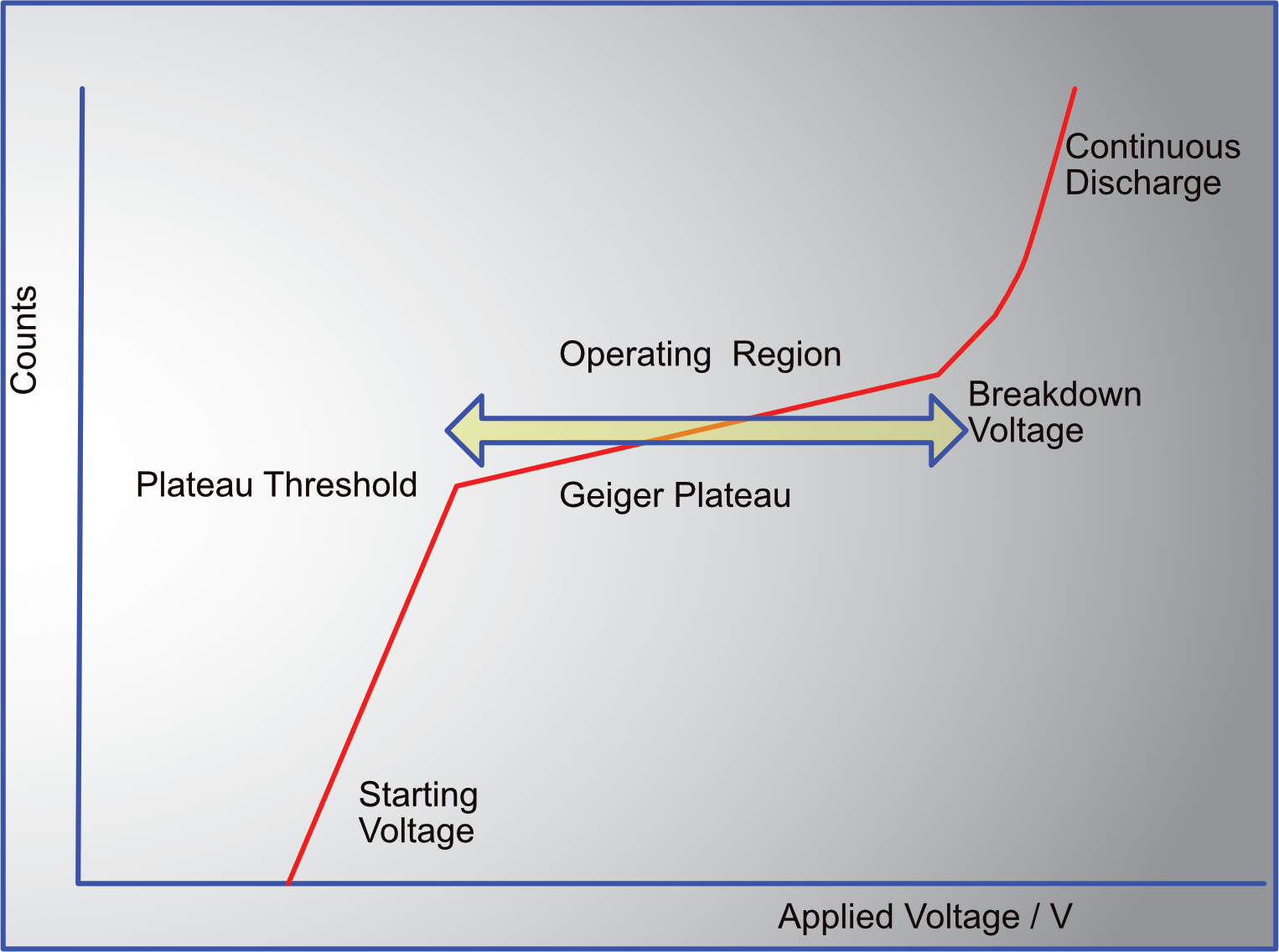
The amount of charge that results is dependent upon the voltage (as shown), which needs to be above the threshold voltage. If we consider there to be a voltage more than this, then amount of charge produced will be proportional to thus excess voltage.
The output signal, which is normally in the order of volts, will be generated by 108 - 1010 ion-pairs. The circuit capacitance also has an impact on the performance, the higher that capacitance then the lower the signal registered for counting.
Usage in EasySense
Connect the sensor to EasySense, use Devices.
Select the counting ranges that is desired (1 s, open, pulse etc).
Go to Setup and select whether a Continuous or Snapshot measurement regime is desired (see below).
Press Start to commence.
Press Stop to terminate collection.
Measurement Strategy
The GM tube offers many analytical capabilities. At of this, it is a counting system. If one decides to do comparative studies across "stable" samples, then considerations of how an average count was are to be achieved should be considered and how long they might take to do. If the system is more temporally dynamic, then sampling time comes into this to achieve a good activity rate (and how it is reported) in conjunction with the dynamics that are being observed.
The Counting Statistics section below gives a guide on how to sample. If there is a high enough signal rate that can be accurately reported, which is short enough compared to the changes that you are recording, then this will be an effective way forward. If the fluctuations in rate are high and one needs a long time to ascertain that data, then rate of decay information, for example, will be less certain.
EasySense offers two useful regimes for data collection with this sensor. Snapshot enables a user to capture a moment of data for sample-to-sample comparisons. Continuous mode streams the data in time so that variations temporally can be mapped.
General Recommendations
Please ensure that the sensor is properly and securely mounted where possible.
Please observe all local safety regulations relating to radiation safety!
Follow the Notices Section
Keep the distance between the source and the GM tube easy to measure and use whole units!
Additionally
- Persons under 16 years of age should not handle any radioactive sources.
- Never handle a source without protection available, or directly.
- Always use tongs or tweezers to manipulate the source.
- Never open a sealed radioactive specimen.
- Keep as much distance from sources as practicable.
- Sources should be secured when not in use.
- Always return the source to its dedicated container after use.
- Keep detailed records of radioactive source usage.
- Report all incidents and accidents immediately using the accepted procedures.
- Never point a source at anyone, including yourself.
- Make sure all radioactive compliance and leakage information is conducted to the correct schedule.
Sensitivity and Percentage Efficiency
The sensitivity of a GM tube depends on two things, once one is in the Geiger plateau for detection. The gas response to an ionising event will impact upon the registered count. Also, the size of the window of a GM tube will be able to accept a certain percentage of the radiation on offer.
For a uniformly radiating source, with a total count rate, N, the counts per unit area, Γ at a distance X from the source will simply be:
Γ = N/(4ΠX2)
The amount of radiation that a GM window will accept is governed by the window area. If the window is round with a radius, r, then the amount that will pass given the above is the ratio of window area to the spherical surface defining the emission of radius, X, where the GM tube window is located.
Window Area = Πr2
There is an emission angle, Θ, that will encase the window dimensions, when the angle is small:
Window Area = Π(Xsin(Θ/2))2
Spherical surface area = 4ΠX2
The collection percentage, ϑ is:
ϑ = Window Area/Surface Area
ϑ = Π(X2sin(Θ/2))2/(4ΠX2)
ϑ = 0.25(sin(Θ))2
If Θ = 4 degrees from a projected radius(X), then ϑ is 0.12%.
The registration of ionising events depends upon the "GM tube sensitivity". The effect of gamma radiation may well be quite different to beta and alpha. If there is a registered activity, Nr, and a percentage efficiency, δ, of those events converted to electron bursts, given that we have a background count, b, we can calculate δ as a percent by:
δ = [(Nr - b)/(ϑN)]*100
Radioactive Decay Formulae
When a source decays, the number of counts per unit time, Nr, can be recorded. If a source is decaying exponentially, then at every half-life, the activity has fallen to 50% of the previous period. With the Geiger tube we can follow this directly. Another way of using the tube is to say that we know the count, Nr, after a defined time but we know the half-life - so what is the initial count, N?
Every t0.5, the count falls to 0.5 of the previous value. So, at the value of t/t0.5, or Ψ, then the count we see is:
N = Nr/(0.5)Ψ
If 4 half-lives have elapsed (Ψ = 4) and the count was 50 CPM (counts per minute), then
N = 50/(0.5)Ψ
N = 50/(0.5)4
N = 800
Another way to express this behaviour is by using a decay constant, λ:
Nr = Nexp(-λt)
with an additional background count rate, b,
Nr = Nexp(-λt) + b
will give the final count rate observed.
The half-life of the event is given by:
(Nr - b)/(N - b) = 0.5 = exp(-λt0.5)
if b is small, t0.5 occurs when it is equal to Nr / N = 0.5 or the product λ t0.5 = -0.693.
Electric Field Considerations
When a defined amount of charge is allowed to become established in a cylinder, an electric field and potential is set up. This can become significant. Using Gauss's Law, the electrical flux, ϕ, can be related to the radius concerned, electrical field strength, E, tube length, L, by the following relationship:
ϕ = E2ΠrL = λL/ε0
and ε0 is the permittivity of free space and λ is the charge per unit length.
therefore:
E = λ /(ε02Πr)
The voltage can be evaluated by the following defining the radius of the inner and outer tubes (ra and rb respectively):
rb
ΔV = ∫ λ /(2Πε0r)dr
ra
ΔV = λ(2Πε0)-1 ln(rb/ra) = λκe ln(rb/ra)
The capacitance of a cylinder, C, can be derived. The total charge, Q, will be:
Q = λL
and since
C = Q/V = 2Πε0L/ln(rb/ra)
thus:
C/L = 2Πε0/ln(rb/ra)
giving the capacitive properties of the GM tube.
GM Tube Recovery Time
The rates of collection for both positive and negative ions are different, the electrons are collected in the microsecond regime, whilst the cathode collects in the millisecond regime.
The field gradient is intense toward the anode. The positive space charge located around the anode briefly prohibits the promotion of further electron avalanches.
In operation, there is a recovery time, τ, For N events, then the recovery is Nτ. When it is running in a time = ~(1 - Nτ) is expended, there are in effect Nr events logged by N registered pulses, given by:
Nr = N(1 - Nτ)-1
Nr effectively becomes equal to N when the tube is in low usage.
The recovery time is influenced by the above and the capacitive characteristics of the tube and the associated electronics.
Counting Statistics
With conditions pertaining to radioactive decay, A distribution function P(x) that is the probability of observing X counts in one observation period can be defined. The distribution of the values Xi about the true average, Xa, is called the Poisson distribution and has the form:
Sample mean:
N
Xa = 1/N Σ Xi
i=1
The sample standard deviation, s:
N
s2 = 1/(N - 1) Σ (Xi - Xa)2
i=1
Population standard deviation:
μ = limit of Xa as N approaches infinity, so N -1 is effectively = N
N
σ2 = 1/N Σ (Xi - μ)2
i=1
or
N
σ = (1/N Σ (Xi - μ)2) 0.5
i=1
The above variance allows us to evaluate whether a particular percentage of the counts fall within this limit. For our distribution, 68% of events lie within the total distribution using plus or minus
σ.
(From P. R. Bevington, Data Reduction and Error Analysis for the Physical Sciences, pp. 10-24.)