The speed of sound and its importance are evident all around us. You may have noticed that a lightning strike and the associated thunder do not coincide. This informs us that speeds involved are different. 

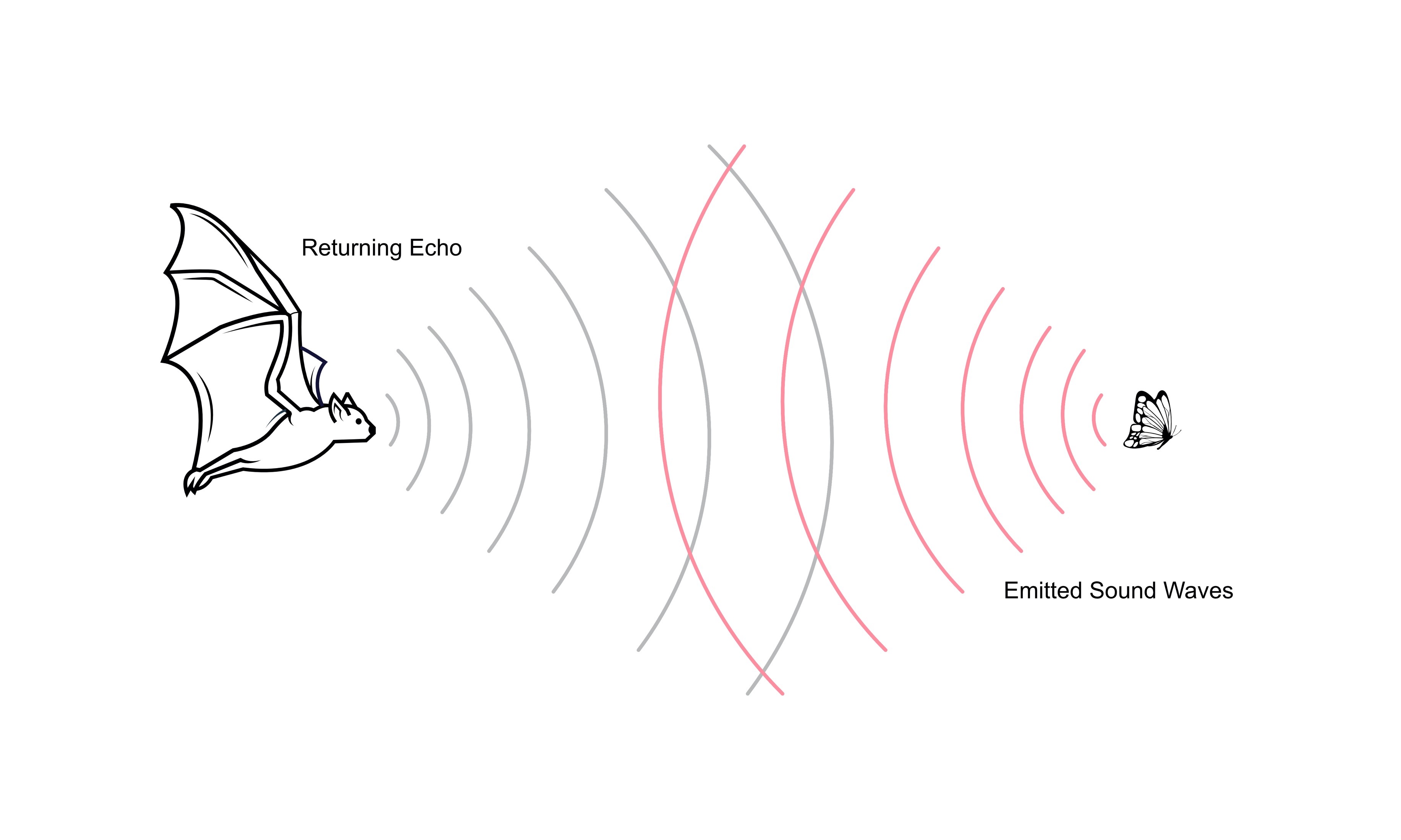
Bats use their fine-tuned sense of sound to navigate around the world: the time delay for the echo they detect is related to the distances involved. This is part of animal echolocation, and animals such as odontocetes (toothed whales) use sonar for these purposes.

William Derham was the first recorded person to measure the speed of sound, in the late 17th / early 18th century. He used a simple method of creating a sound wave and measuring how quickly it reached two points. Knowing the distance separating these points and the time taken to reach them, the observer could calculate the speed of sound. The experiments described in Data Harvest's associated practical work sheets use a method similar to that used by William Derham.

Modern technology reduces the distance between the "listening points". With two microphones at a known distance apart, the time taken for that noise to travel between microphones is a direct link to the speed of sound. A simple calculation of distance divided by time gives the speed. Since the sound profile is known, we can analyse the experiment in diverse ways, and are not reliant upon interpretation of when a wave front arrives at one point or another. Alternatively, following a sound wave "bouncing" back and forth from one surface to another gives a frequency. This characteristic frequency, when analysed, provides another way to measure the speed of sound. 

Sound Propagation

Sound is a vibration that travels through an elastic substance. The vibration causes areas of compression and expansion forming a longitudinal wave, which can show properties of reflection. 

As a rule, the greater the elastic properties of a material the faster the speed of sound, c. In air (a mixture of gases) at a temperature of 0ºC, sound travels at 331 metres per second. As the temperature increases the speed also increases (by approximately 0.607 m s-1 ºC-1). The speed of sound in air is independent of pressure and density for small temperature ranges. 

Speed travels about four times faster in water than air and this multiple is temperature dependant. In solids additional waves related with shear and extensional modes may also be present. These additional waves can lead to widely varying speed values cited in the literature. 

Speed of Sound Value and Transit Time 

Values are at 1 atmosphere 25 0C, Source-engineeringtoolbox.com

The quoted speed of sound in air value is often a calculated rather than by direct measurement. The formula used to calculate the speed of sound in air produces satisfactory results over a wide range of temperatures but starts to fail at elevated temperatures. Good predictions of the speed of sound in the atmosphere are possible, especially in the colder, drier, low-pressure stratosphere. 

When longitudinal waves are present - the disturbance travels in the same direction as the sound. In solids, the picture is often more complex as shear waves can also be present. The vibrations of these are at right angles to the sound propagation. Extensional mode waves travel as above, which can contribute. 

Measurement Strategy

Sound is a disturbance moving through a media. If it can only travel as a unidirectional pulse (longitudinal) then, we can measure the time taken for it to travel a certain distance. This is the "time-of-flight". This will be the case in gases, fluids and with longer distance measurements involving solids.

Solids can support more complex modes of propagation (see above). Transverse waves are usually slower than longitudinal waves. They do not progress at an interface (say an air boundary) and convert back to their longitudinal alternative. With no interface, one can make use of time-of-flight across the material. If the sound wave encounters two interfaces, such as air at either end, then it will "bounce back" and resonate, or ring. Here we can use resonance analysis to map the speed of sound, such as that exhibited in a short metal rod.

Usage in EasySense

1. Connect the microphones to the sensor unit and turn on.

2. Activate your EasySense app and select Devices. Connect the sensor.

3. In the Devices dialogue, select the data that you wish to display. 

    The parameters that are relevant for your experiment, you selected here.

3. Select Continuous, Interval required, pre-trigger (Start) and Stop sample number needed. 

4. Start to initiate experimentation.

General Recommendations

1.   Do not expose the microphones directly to water. 

2.   If clamping the microphones, apply only a gently pressure.

3.   For long "time-of-flight" studies, employ a 4 mm jack extension cable (not supplied).

4.   Please observe the Notices Section in this document.

Usage Recommendations for Air

1.   Use 1.0 m to separate the microphones. 

2.   Position the microphones so that they are at right angles to the sound propagation.

3.   Arrange so that you create the noise behind the first microphone (A). 

4.   Try to use a dedicated device to generate the disturbance.

      For air, an inexpensive fast "clicker" is ideal to generate a sound wave. 

5.   Try to isolate any sound-reflecting surfaces from the experiment. 

6    Should you wish to explore supersonic behaviour, try using a balloon burst! 

7.   Using Setup, select Start "When Value Rises Above" and set default conditions there.

      A pre-trigger delay and fixed number of samples "Stop" condition work well. 

Specific Usage Recommendations for Solids (Metals)

Trying to invoke sound in sections of metal can come with problems. Mechanical generation of sound will set off a complex series of vibration modes that can be difficult to differentiate. To simplify experimental behaviour, however, we recommend the following.

Time-of-flight (long section) 

1.  Use a long piece of metal (fence, stair rail) > 5 m for time-of-flight. 

     In this mode the microphones effectively function as accelerometers.

2.  Use a small hammer, and record the disturbance arrival times at A and B. 

     The equation below may then be used, after analysis, to calculate the speed of sound. 

3.  Try using "G" clamps to hold the microphone gently against the surface.

4.  Use a software trigger available from the Setup dialogue.

     Try using a pre-delay of fifty microseconds and a few milliseconds data gathering. 

5.  Select Start "Value Rises Above" and set default conditions there.

6.  A pre-trigger delay and fixed number of samples Stop condition work well.

7.  Use the fastest interval possible.

Resonance studies (short section)

1.  For resonance, use a metal rod > 1 m with diameter circa 10 mm.

2.  Try not to use rolled metal. 

3.  Suspend the rod, at either end, using elastic straps attached to a supporting rod.

     A ribbon attached to the centre of the rod can dampen half-wave harmonics.

3.  Use a light hammer, face on, to generate the resonance.

4.  To help understand the calculations, try to use ‘sensible’ sections, e.g., 1 m.

5.  Use a software trigger, if possible, available from the Setup dialogue (above).

     Select Start "Value Rises Above" and set default conditions there.

6.  A pre-trigger delay and fixed number of samples Stop condition work well.

7.  Use the fastest interval possible.

Theory

The mathematics behind sound advancement are quite accessible. The speed of sound, c, is expressed:

      c = √ (Ep /ρ)

where Ep is a measure of the elastic properties and ρ is the density. 

Gas

The speed of sound c is a result of compression waves. With an ideal gas:

      c = √(γRT/m)

here γ is the ratio of the specific heat capacities (Cp/CV) and m is the molar mass of the gas (kg mol-1)   

or: 

      c = √(γkT/m0)

where m0 is the molecular mass of the gas molecule(s) involved (kg). 

Setting γ = Cp/Cv = 1.4, R = 8.3 J mol-1 K-1, m = 2.9 × 10 -2 kg mol-1, T = 273 K, c is 327 m s-1.

Also, the speed of sound is related to the average speed of diatomic gas molecules, c1:

     c1 = √(3kT/m0)

For nitrogen (m0 = 4.64×10 -26 kg), at 273 K, c1 is 493 m s-1.

or: 

     c1 = c × (γ/3)-0.5 

   

which is a remarkably interesting relationship to have!

    

Liquid

With a liquid, shear forces are not available and so we may express the speed of sound:

     c = √(B/ ρ)

where B is the bulk modulus. The Bulk modulus is a way to express the reduction in volume of a fluid with an applied pressure. For water, B = 2 GPa or 2 × 109 kg m s-2, ρ = 1 × 103 kg m-3, yields a value of c = 1000 m s-1.

Solid

The situation is a little more complex in a solid, as both compression and transverse waves can make up the speed of sound (see above). Transverse waves oscillate in a direction which is perpendicular to the direction in which the wave is advancing. 

Solids support elastic deformation: compression waves travel at different speeds to the transverse wave. During an earthquake, what is often experienced is the initial shock and then the rocking behaviour exhibited by transverse waves comes a little after the first compression wave.

A flat surface, such as a bench top, will contain different velocities and wave echoes. The cross section (and area) of the material will also have an influence. 

If the solid is a flat rod, then the velocity of sound will be dependent upon the shear and Young's modulus of the material. In the case of a shear wave:

    c = √(G/ ρ)

where G is shear modulus. For steel, G = 210 GPa or 2 × 1011 kg m s-2, ρ = 8 × 103 kg m-3, yields a value for c = 5 × 103 m s-1. Shear waves cannot progress when they enter a boundary such as air and convert back to longitudinal waves.

In the case that the speed measured as a longitudinal wave pressure front dominates, the above reduces to:

    c = √(E/ ρ)

and E is Young's modulus. 

Long section (>4 m) "time of flight"

We can measure the time separation for a sound disturbance front, when the longitudinal wave is cleanly separated from effects of shear, reflection, and other more advanced modes in the following. This would apply to a sample that is long enough to easily detect the oncoming front.

If one has a large separation, l, between the microphones and the sound transmission is unidirectional, the speed of sound (fastest) is the rate measured when separation between initial pulse front (location A) progresses to location B, with a time-of-flight, t, resulting in:

     c = l/t

By measuring across a large separation between the microphones, we can estimate the speed of sound.

Short section (1 m) "resonance"

The speed of sound (longitudinal) along a rod or bar of length, l, will exhibit a major frequency, f. The longitudinal pulse can bounce back and forth but also impart its frequency to the air when it encounters an air interface. This is true when the diameter of the bar is insignificant compared to the overall length. These quantities are related by the formulae: 

     c = 2 × l × f                                                                                                                                  *

The characteristic (major) frequency is:

     f = 0.5 × l-1 × c

  

     f = 0.5 × l-1√(E/ ρ)   

For steel, E = 210 GPa or 2.1 × 1011 kg m s-2, ρ = 8 × 103 kg m-3,  yields c = 5 × 103 m s-1. The major frequency for a rod of length 1 m, is 2.5 ×103 s-1 or 2.5 kHz. 

Over a short distance, using a rod of 1 m, we can employ this method to find the value of c. One can examine the characteristic ringing that results when a metal is set into vibrational excitation governed by the speed of sound

Useful Formulae

The following formulae, are particularly useful: 

   

    speed = distance travelled/time elapsed

    wavelength = speed/frequency 

or 

     speed = wavelength × frequency 

For a resonating rod, longitudinal mode: 

     wavelength = 2 × length of rod       

     speed of sound = 2 × length of rod × frequency   

Faster than sound....

When a disturbance travels faster than sound, we say that it is supersonic. The Mach number, M, is a value quoted for the ratio of speed of flow velocity, u, compared to the local speed of sound, c, in a particular medium.

     M = u/c  

This type of energy propagation is different from when sound alone carries the disturbance. Shock waves manifest in diverse forms, from aircraft "breaking the sound barrier", earthquakes and volcanic eruptions and meteor strikes.